
Vishnu Ravendranathan
Wednesday, June 18, 2025 | 15 minutes
Teaching a Ship (model) to Learn: From Classical Rules to Reinforcement Learning
TL;DR: Phase 1 gave us a classical navigation system that works. Phase 2 asked a harder question: can a neural network learn to navigate without being told the rules? Short answer: yes, sort of. It’s faster. It’s sometimes smarter. It also runs aground in ways a trained officer never would. Here’s what six months of RL training taught me about autonomous ships, and about the limits of learning from scratch.
Where We Left Off
If you read Part 1, you know where we ended up: a working classical pipeline with A*, ILOS path following, and a COLREGs-aware collision avoider. It had rough edges. The vessel occasionally ran aground when dodging multiple threats. Path resumption was clunky. But it worked, and every decision it made was explainable.
Phase 2 question: can reinforcement learning do better, and can we understand what it’s doing?
Spoiler: it does some things better, some things worse, and the combination of both is probably the answer.
Before RL: Upgrading the Physics
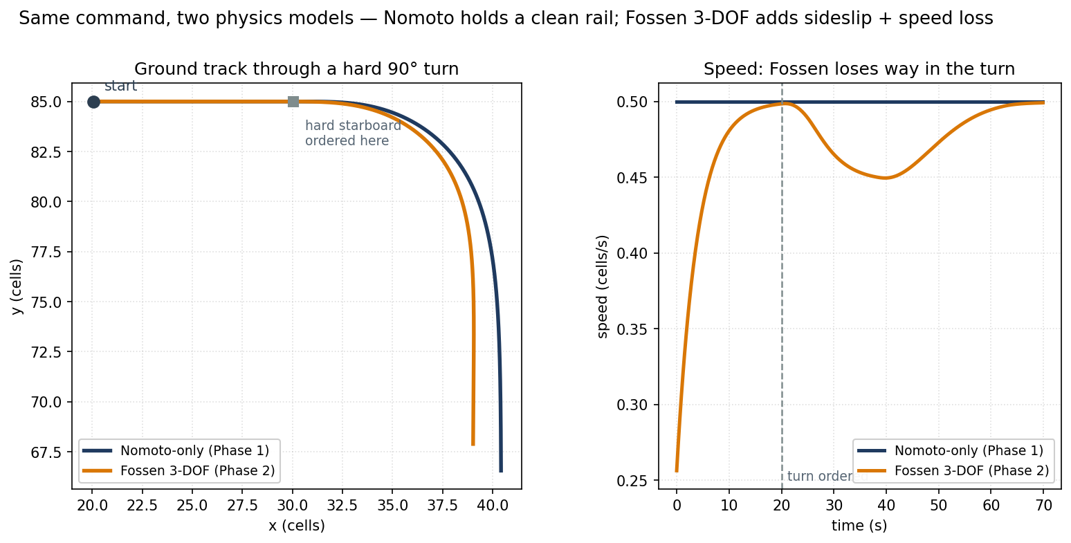
Before training anything, I had to fix the simulator. The Nomoto first-order model from Phase 1 was fine for visualization, but it had one problem: it only modelled yaw (turning). The vessel had no sideslip, no turn-induced speed loss, no environmental forces. It behaved like a ship on rails.
The fix: Fossen’s 3-DOF maneuvering model.
Three degrees of freedom means the vessel now has coupled dynamics across surge (forward and back), sway (sideways drift), and yaw (heading). In practice this means:
- When the ship turns hard, it drifts sideways a little. That’s sideslip, like a car cornering but not quite a drift.
- Hard turns bleed speed too. That’s turn-induced speed loss, the more rudder, the more drag.
- Water current and wind gusts apply forces directly to the vessel, pushing it off course even when it’s doing nothing wrong.
In plain terms, before any of the math, this is what the update does every tick:
surge_accel = -drag * (surge_speed - reference_speed)
sway_accel  = -sway_drag * sway_speed - sideslip_coupling * surge_speed * yaw_rate
yaw_accel   = (1 / time_constant) * (-yaw_rate + gain * rudder_angle)

Where:
drag                 = how fast surge speed settles back to the reference speed
sideslip_coupling    = how much the yaw rate drags the ship sideways
time_constant, gain  = the same T and K from the Nomoto model in Phase 1
Written out properly, the surge equation pulls speed back toward a reference value:
$$ \frac{du(t)}{dt} = -X_u\big(u(t) - u_{ref}\big) $$
The sway equation is where the sideslip comes from. It couples lateral drift to the yaw rate:
$$ \frac{dv(t)}{dt} = -Y_v v(t) - Y_{vr} u(t) r(t) $$
Yaw still follows the same Nomoto first-order form from Phase 1, it never went away, it’s just one piece of a bigger model now:
$$ T \frac{d r(t)}{d t} + r(t) = K \delta(t) $$
Environmental forces (current, wind) get resolved into the vessel’s body frame and added directly to the surge and sway accelerations each step:
$$ u_c = V_{c,x}\cos\psi + V_{c,y}\sin\psi, \qquad v_c = -V_{c,x}\sin\psi + V_{c,y}\cos\psi $$
where $\psi$ is heading and $V_{c,x}$, $V_{c,y}$ are the current and wind velocity components in the world frame. $u_c$ and $v_c$ get added straight onto the surge and sway accelerations above.
And here’s the same thing as actual code, the lines map directly onto the equations above:
# Simplified 3-DOF update (Fossen linear maneuvering)
# Maps to: du/dt, dv/dt, dr/dt from the equations above, plus u_c/v_c for current and wind

# du/dt: surge acceleration
du = -self.xu * u + self.xu * self.u_ref  # drag towards reference speed

# dv/dt: sway (sideslip), coupled to yaw rate
dv = -self.yv * v - self.sideslip_gain * u * r

# dr/dt: yaw acceleration, Nomoto form
dr = (1.0 / self.T) * (-r + self.K * delta)

# Environmental forces
du += current_x * cos(heading) + current_y * sin(heading)
dv += -current_x * sin(heading) + current_y * cos(heading)
The result looks more like a real ship. It overshoots turns slightly. It drifts in crosscurrents. And every agent in the simulator runs through this same physics: classical, MPC, RL, one engine, no exceptions. That matters a lot when you’re comparing results later.
Building the RL Environment
For RL to work, you need three things: what the agent sees (observation), what it can do (action), and what motivates it (reward). Getting all three right is harder than it sounds.
What the Agent Sees
I used Gymnasium (the modern successor to OpenAI Gym) to wrap the simulator. The observation vector has 35 features:
observation = [
    # Goal: where are we trying to go?
    goal_bearing,          # angle to goal, relative to heading
    goal_distance,         # how far away

    # Own state
    surge_speed,           # forward speed
    yaw_rate,              # how fast we're turning
    heading_sin,           # sin/cos encode heading without wraparound issues
    heading_cos,

    # 16-ray land lidar: one range reading per compass sector
    *lidar_ranges,         # 16 values: distance to nearest obstacle in each direction

    # 3 nearest traffic vessels (× 3)
    *[bearing_i, distance_i, closing_speed_i for each vessel]
]
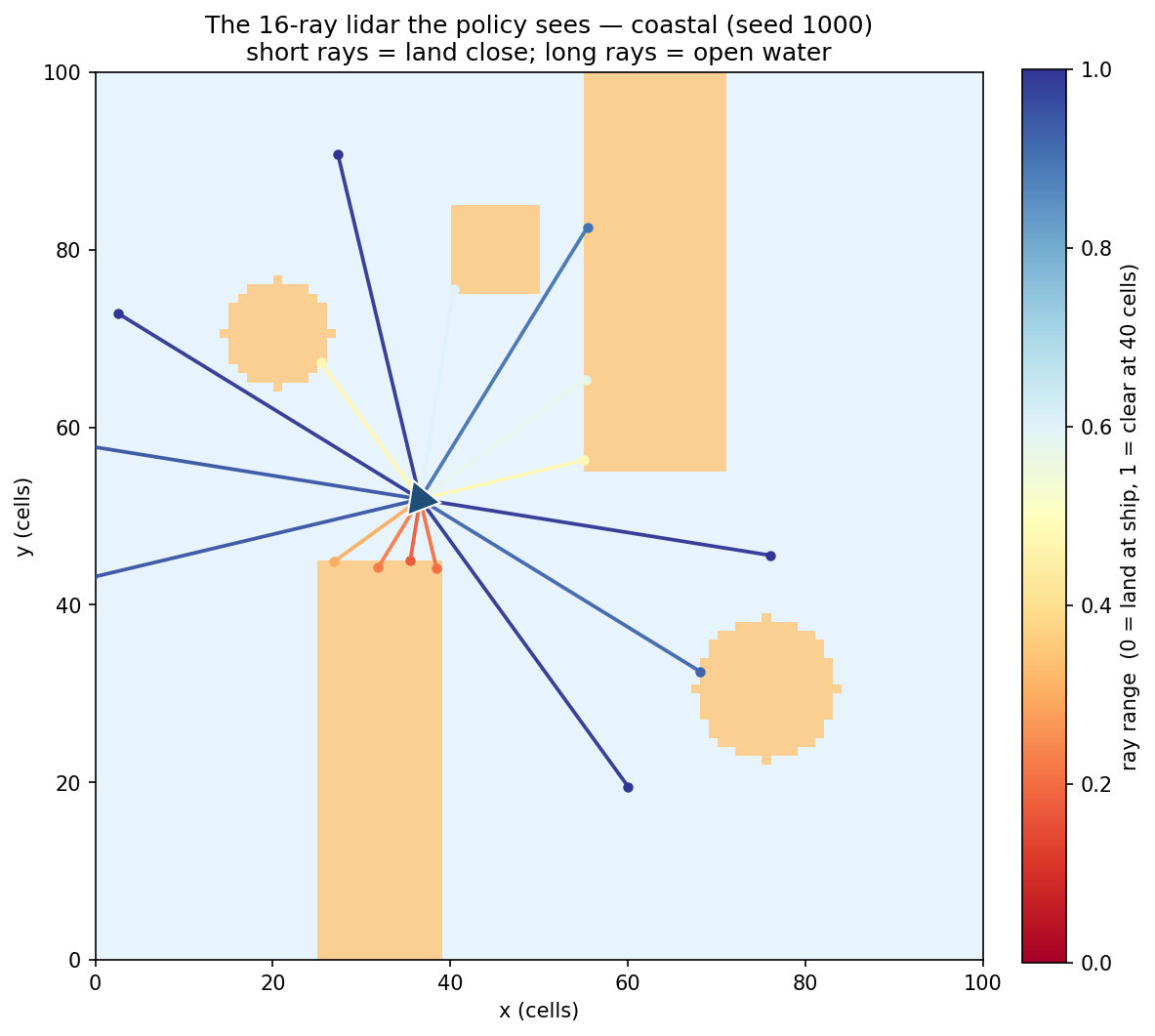
The 16-ray lidar was the most important design decision. Without it, the RL agent has no sense of where land is except by crashing into it. With it, it develops something that looks almost like spatial awareness. You can watch it slide around coastlines with a confidence that’s slightly eerie.
What the Agent Can Do
The action space is discrete: course change offsets relative to current heading. Options like −30°, −15°, −5°, 0°, +5°, +15°, +30°. Each action is held for several simulator steps, an “action repeat”, before the agent chooses again.
Why discrete and why action repeat? Two reasons. First, it matches the abstraction level of the classical agent, a “helm order”, so comparing them later is apples to apples. Second, continuous action spaces with PPO on this task led to very jittery, unrealistic helm behaviour during early training. The agent would oscillate the rudder continuously. Discrete actions plus action repeat force it to commit to a decision.
What Motivates It
Reward design is where I spent the most time and made the most mistakes.
The final decomposition is:
$$ R_t = w_p \Delta d_t - c_\tau - c_n \mathbb{1}\left[d_{min,t} < d_{thresh}\right] $$
On top of that, a terminal bonus or penalty gets added once the episode ends, success, collision, grounding, or timeout each carry their own fixed reward, exactly as you’d expect from the code below.
In code:
# Every step
reward += progress_reward      # reduction in distance to goal (positive)
reward -= time_penalty         # small constant negative (encourages efficiency)
reward -= near_miss_penalty    # if min_separation < threshold

# Terminal
if success:    reward += 100.0
if collision:  reward -= 80.0
if grounding:  reward -= 80.0
if timeout:    reward -= 20.0
The key lesson: every component is logged separately, every step. When training went wrong, which it did, multiple times, I could see which component was driving the bad behaviour.
Early versions of the reward function produced an agent that learned to spin in tight circles. It avoided the time penalty by moving, avoided the near-miss penalty by staying away from everything, and never reached the goal. The progress term fixed this, but it took me two full training runs to figure out why it was spinning.
Training: PPO and the Long Wait
I used PPO (Proximal Policy Optimisation) via Stable-Baselines3. No custom implementation, SB3 is battle-tested and the training loop basically writes itself:
PPO optimises a clipped surrogate objective so policy updates don’t move too far from the previous policy in one step:
$$ L^{CLIP}(\theta) = \mathbb{E}\Big[\min\big(r_t(\theta) A_t,\ \operatorname{clip}(r_t(\theta), 1-\epsilon, 1+\epsilon) A_t\big)\Big] $$
$$ r_t(\theta) = \frac{\pi_\theta(a_t \mid s_t)}{\pi_{\theta_{old}}(a_t \mid s_t)} $$
$r_t(\theta)$ is the probability ratio between the new and old policy for the action actually taken, and $A_t$ is the estimated advantage at that timestep. The clip term stops a single batch of good (or lucky) episodes from swinging the policy too far in one update.
from stable_baselines3 import PPO
from stable_baselines3.common.env_util import make_vec_env

env = make_vec_env(VesselNavEnv, n_envs=4)  # 4 parallel environments

model = PPO(
    "MlpPolicy",
    env,
    learning_rate=3e-4,
    n_steps=2048,
    batch_size=64,
    verbose=1,
    tensorboard_log="./logs/"
)

model.learn(total_timesteps=10_000_000)
model.save("models/ppo_vessel")
“The training loop writes itself” is true. Understanding what’s happening during training is a different story.
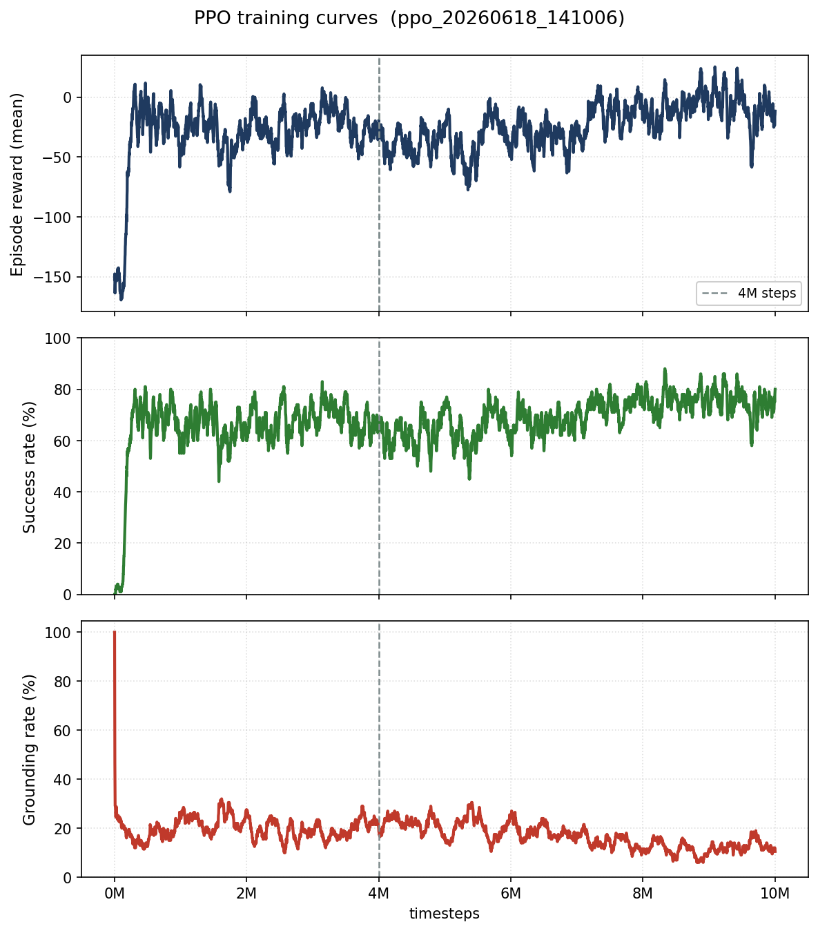
What 4 Million Steps Looks Like
Around 4M steps, the policy starts to look competent. It navigates clean open water confidently. It avoids obvious traffic. It reaches the goal more often than not.
But it runs aground. Not always, not even usually, but about 13.3% of the time in the benchmark suite, it finds a landmass and parks itself into it. Specifically: landmass geometries it hadn’t seen much during training. The coastal scenario. Narrow channels. Random islands with unusual shapes.
This is the generalisation gap. The policy learned to navigate the environments it trained in. Maritime geography is diverse, and a neural network trained on one shape of coastline doesn’t automatically generalise to a different one.
What 10 Million Steps Looks Like
I expected doubling the training budget to close this gap. It didn’t. Not meaningfully.
| 4M steps | 10M steps | |
|---|---|---|
| Score | 74.6 | 75.5 |
| Success | 76.2% | 76.7% |
| Grounding | 13.3% | 12.2% |
| COLREGs compliance | 0.63 | 0.64 |
+0.9 score point. −1.1pp grounding. +0.01 compliance. The policy improved, but barely. It had reached the ceiling of what it could extract from the current training setup.
This was the clearest signal that the problem isn’t training budget, it’s the diversity of training scenarios. The policy needs to see more coast shapes, more confined geometries, during training. That’s a curriculum learning problem, not a compute problem.
How RL Actually Behaves vs. Classical
This is the most interesting part. Watch both agents navigate the same scenario and you immediately see the personality difference.
Classical moves like a cautious senior officer. It plans its route, follows it carefully, responds to traffic with early and deliberate alterations, and resumes the route cleanly after the threat passes. Every decision has a reason you can read in the decision log. It takes 224.9 seconds on average to complete a scenario.
RL moves like a very confident junior officer who cuts corners. It finds shorter paths, path efficiency of 1.00, meaning it routinely beats the planned route length. It completes scenarios in 197.4 seconds on average, 12% faster. But its COLREGs compliance is 0.64 versus classical’s 0.94. It sometimes turns the wrong way in head-on situations (compliance 0.33 on Rule 14, the head-on rule).
It’s not subtle on video. Classical sees the head-on contact and commits early to a clean starboard turn. RL hesitates, sometimes picks the wrong side, and corrects late.
Rule 15, the crossing rule, tells the same story from a different angle. When another vessel is crossing from our starboard side, we’re the give-way vessel and the rule expects an early, substantial turn.
Classical gives way early and obviously. RL gives way too, eventually, but the turn comes later and reads as reactive rather than deliberate, even when it technically avoids the other vessel.
There’s something almost characterful about it. In open water it’s decisive and efficient. Near coastlines it occasionally freezes into a bad trajectory and commits. In multi-vessel situations it sometimes makes unconventional choices that happen to work out, and sometimes don’t.
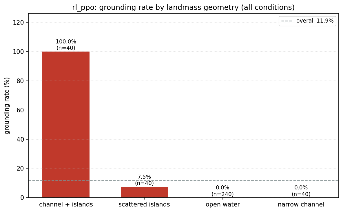
The Grounding Problem, Specifically
Groundings happen at landmass geometries underrepresented during training. The agent has learned to navigate around the types of islands it saw during training. Novel shapes, particularly long, thin peninsulas or concave bays, sometimes fool it. The lidar rays see the obstacle, but the policy hasn’t learned the right evasion for that shape.
Classical doesn’t have this problem because A* replans explicitly around whatever geometry is in the grid. It doesn’t need to have “seen” a shape before. RL pattern-matches. Classical reasons.
The Shielding Insight
This was the finding that changed how I think about the whole problem.
What if you let RL navigate, but put the classical safety checker on top? Every time the RL policy proposes an action, run the classical predictive avoider’s rollout. If the proposed action leads to a grounding or collision within the horizon, substitute the nearest safe alternative instead.
$$ a_t = a_t^{RL} \text{ if rollout}(s_t, a_t^{RL}, H) \text{ is collision-free and grounding-free, otherwise } a_t^{classical} $$
Result: groundings go from 12.2% to zero. Completely eliminated. The RL policy still drives, it’s still fast, still finds short paths, but it can’t commit a fatal mistake because the classical layer catches it.
This is called shielding, and it’s an active area of safety research. What I found is that it costs about 11 additional seconds per scenario (208.8s vs 197.4s for unshielded RL), the price you pay for the classical layer’s more conservative substitutions. But it’s zero-grounding with decent COLREGs compliance (0.67 vs 0.64 unshielded).
It’s the most practical finding in this whole project. Pure RL isn’t ready to be alone on the bridge. Classical alone is slow and rigid. The combination gets you most of the benefits of both.
The COLREGs Problem Neither Approach Fully Solves
Here’s something I didn’t expect: both classical and RL score 0.76 on COLREGs Rule 17 (stand-on, crossing-from-port situation). So does MPC. So does the shielded hybrid.
Rule 17 (simplified) says: if you have right of way, maintain your course and speed. The vessel crossing from your port side should keep clear of you. For those who want to refresh the full text, it’s here: https://ecolregs.com

Every approach I tested responds by taking early evasive action instead of holding. This is safer in absolute terms, you avoid a close-quarters situation entirely, but it’s technically non-compliant. A human officer on the other vessel, who is expecting you to hold your course as required by the rules, now has to deal with your unexpected alteration.
The classical agent is non-compliant here because the cost function for the avoider penalises proximity. The RL agent is non-compliant because nothing in the reward function specifically rewards holding course. It just rewards not colliding. Any cost function that penalises proximity will tend to produce Rule 17 non-compliance, because holding course when another vessel is approaching looks, locally, like a bad move.
This is a fundamental tension. It matters for autonomous vessel certification. I’ll be exploring it further.
What I Got Wrong (A Non-Exhaustive List)
- First reward function: produced a spinning agent that avoided the time penalty by moving without going anywhere useful
- Second reward function: collision penalty too small, agent learned to brush obstacles lightly (technically not a collision by threshold) rather than avoid
- Continuous action space: led to jittery, unrealistic helm behaviour, switched to discrete
- No action repeat: agent made a new decision every physics tick, which is both unrealistic and makes learning harder, too much noise
- Training on too few scenario types: the generalisation gap is entirely my fault, I could have used curriculum learning from the start
- Expecting 10M steps to fix the generalisation gap: it doesn’t. More training on the same scenarios makes you better at those scenarios, not different ones.
What’s Actually Impressive About RL
Despite the problems, some things are genuinely impressive:
It finds shorter paths. The classical agent follows the A* planned route. RL ignores the route and navigates directly. In practice it beats planned route length consistently (path efficiency 1.00), at the cost of safety.
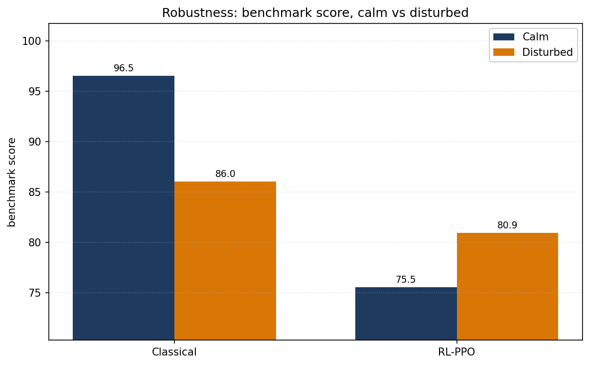
It degrades gracefully under disturbances. In disturbed conditions (current and wind gusts), the RL policy’s score actually improves (score 75.5 calm to 80.9 disturbed), likely because the disturbances affect its competitors more than itself. The classical pipeline scores drop more sharply (96.5 to 86.0) because the ILOS integral correction lags under rapid disturbance changes.
It learned COLREGs-ish behaviour without being told. Nobody programmed “turn to starboard in a head-on situation” into the RL agent. The reward signal includes a weak COLREGs preference term, but the bulk of compliance came from experience. It learned that starboard turns in crossing situations tend to lead to better outcomes. Not perfect, compliance is 0.64 overall, but genuinely emergent.
AI-Assisted, Round Two
I cant math without help, calculators to blame. Claude Code was my buddy for most of this project: scaffolding the Gymnasium environment, debugging, writing the PPO training scripts, and explaining the shielding literature I was reading for the first time. It didn’t decide what “good” COLREGs compliance looks like, which reward terms mattered, or whether x% grounding was acceptable to report honestly instead of hiding. Those calls, and ofcourse every mistake in the list above, are mine.
What’s Next
I’m not done. Two things are in progress:
Closing the generalisation gap. This means curriculum learning: start with simple open-water scenarios, progressively introduce more complex geometries, and make sure the training distribution covers the long tail of coastal shapes. The 10M-step plateau told me clearly that more compute on the same curriculum won’t cut it.
Quantifying the comparison properly. I want to put both approaches through a rigorous, reproducible evaluation. Same scenarios, same seeds, same physics, same metrics for everyone. That’s what Part 3 will be about. Stay tuned.
The code is on GitHub as always: autonomous-vessel-navigation. The RL model weights are in /models/. You can replay any logged episode with python main.py replay logs/your_episode.jsonl and inspect every decision the agent made.
Clone it. Break it. Tell me what you find.
References
- Fossen, T.I. (2011). Handbook of Marine Craft Hydrodynamics and Motion Control. Wiley.
- Schulman, J. et al. (2017). Proximal policy optimization algorithms. arXiv:1707.06347.
- Raffin, A. et al. (2021). Stable-Baselines3: Reliable reinforcement learning implementations. JMLR, 22(268).
- Alshiekh, M. et al. (2018). Safe reinforcement learning via shielding. AAAI-18, pp. 2669-2678.
- Caharija, W. et al. (2016). Integral LOS guidance and control of underactuated marine vehicles. IEEE TCST, 24(5).
- Towers, M. et al. (2024). Gymnasium: A standard interface for reinforcement learning environments. arXiv:2407.17032.