A Sailor's Journey into Autonomous Navigation

TL;DR: I spent the last few weeks building an autonomous vessel navigation system from scratch using Python. Started with basic pathfinding (A*), added realistic ship physics, implemented collision detection and avoidance following COLREGs principles, and got it working with multiple moving vessels. It’s messy, it’s imperfect, but it works. This is Phase 1 - the classical approach. Next up: machine learning. Here’s everything I learned, the bugs I battled, and why this matters for maritime’s future.

But Why?

This year has been about pushing boundaries - IoT solutions, AI projects with MCP, agentic frameworks, and now this: autonomous vessel navigation.

The spark? A couple of research papers on autonomous vessels caught my attention. Reading about CPA/TCPA calculations and COLREGs-compliant avoidance algorithms, I thought: “I understand this from a navigation perspective, but can I actually build it?”

Turns out, you can learn almost anything these days if you’re willing to get your hands dirty. AI tools make the learning curve less painful. I’d done some work with Dijkstra’s algorithm before, so A* felt like the next logical step. But the real aha moment? Learning isn’t gatekept anymore. You don’t need a CS/ML/AI/DS (did i miss something?) degree or to be in a specific geography. You need curiosity and time.

Also, autonomous navigation is coming. Not maybe, not someday - it’s here. I wanted to understand it from the inside, not just read whitepapers about it.

The Game Plan: Classical First, Then ML

The project breaks into two phases:

Phase 1 (this blog): Classical navigation

• A* pathfinding for route planning
• Realistic ship physics (because ships don’t turn or brake like cars)
• Collision detection using CPA/TCPA (maritime standard)
• Collision avoidance following COLREGs principles (well almost)

Phase 2 (coming next): Machine learning

• Train an RL agent to navigate
• Compare classical vs ML approaches
• Figure out the black box problem (especially for COLREGs compliance)

Why this order? You need a baseline. Can’t evaluate if ML is better if you don’t know what “good” looks like. Plus, building the classical system teaches you what the ML agent needs to learn.

Stage 1: The Grid World - Where Ships Live

First problem: how do you represent an ocean in code?

Answer: a grid. Think of it like Excel cells, but each cell is 10 meters of ocean.

class GridWorld:
    def __init__(self, width=100, height=100, cell_size=10.0):
        self.grid = zeros(height, width)  # 0 = water, 1 = obstacle
        
    def add_obstacle(self, x, y, width, height):
        self.grid[y:y+height, x:x+width] = 1.0  # Mark as obstacle

Simple. Islands? Mark those cells as 1. Shallow water? Mark as 1. Restricted zones? Mark as 1.

This felt basic at first, but here’s the thing: this representation works for both classical algorithms AND machine learning later. The ML agent will “see” this same grid.

Stage 2: A* Pathfinding - Finding the Way

You’ve probably heard of Dijkstra’s algorithm - it finds the shortest path by exploring everywhere equally. A* is smarter: it explores more in the direction of the goal.

The key insight: A* uses a heuristic - an educated guess about which direction is promising.

# Simplified A* logic
f_cost = g_cost + h_cost
# where:
# g_cost = actual distance traveled so far
# h_cost = estimated distance to goal (heuristic)

Think of it like this: if you’re navigating from Mumbai to Singapore, you don’t explore routes going towards Europe first. You bias towards Southeast. That’s the heuristic.

Watching A* explore the grid is hypnotic. It spreads out from the start, but heavily favors paths toward the goal. When it hits an obstacle, it flows around it like water.

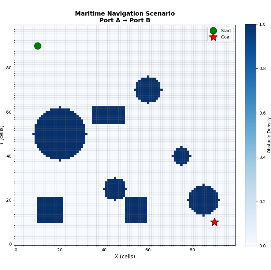
The result? A list of waypoints from Port A to Port B, avoiding all static obstacles.

path = astar.find_path(start=(10, 90), goal=(90, 10))
# Returns: [(10,90), (12,89), (14,88), ..., (90,10)]

Key learning: The path is jagged because it follows grid cells. We’ll fix this later with path smoothing.

Stage 3: Ship Physics - They Don’t Turn Like Cars

Here’s where it got real. A path is just a list of coordinates. How does the ship actually follow it?

Ships have momentum. They don’t turn instantly. When you put the rudder hard over, it takes time for the turn to develop.

Enter the Nomoto model - the maritime industry standard for ship turning dynamics:

T * (rate_of_turn_change) + turn_rate = K * rudder_angle

Where:
K = how responsive the ship is (gain)
T = how long it takes to respond (time constant)

Mathematically, it’s expressed as:

$$ T \frac{d r(t)}{d t} + r(t) = K \delta(t) $$

For a container ship: K might be 0.3-0.5, T might be 30-100 seconds. For our simulation: K=0.5, T=3.0 seconds (faster for visualization).

Nomoto Model Process

Why this matters: When you tell the ship “turn to 45 degrees,” it doesn’t snap to 45 degrees. It gradually builds the turn rate, then gradually reduces it as it approaches the target heading. Just like a real ship.

You can see the difference: the ship can’t make sharp 90-degree turns at waypoints. It overshoots, then corrects. This is physics working.

Stage 4: Path Following - The Steering Brain

Okay, we have a path. We have physics. But how does the ship know where to aim?

Two controllers I implemented:

Pure Pursuit

Look ahead on the path by a fixed distance (say, 50 meters), aim for that point.

lookahead_point = find_point_at_distance(current_pos, path, lookahead=50m)
desired_heading = angle_to(lookahead_point)

Analogy: When you’re cycling, you don’t look at the ground right in front. You look 5-10 meters ahead. Your body naturally steers toward where you’re looking.

Line-of-Sight (LOS)

Maritime standard. Project your position onto the path, then look ahead from there.

closest_point_on_path = project(vessel_pos, path_segment)
target = closest_point_on_path + lookahead * path_direction

The surprising part: LOS was way better at keeping the vessel close to the planned path. Pure Pursuit cuts corners more. For maritime navigation where you might have obstacles near the path, LOS is the way to go.

While trying to improve the manoeuvering, I realised ILOS (Integrated Line of Sight) controller did a better job. ILOS adds an integral term to correct for persistent errors, such as a drift caused by wind or current.

Ok, the math part looks simple but it took me longer than expected to get my head around, but AI helped me understand it better. The cross-track error $y_e$ is the perpendicular distance from the vessel position $(x_v, y_v)$ to the path segment, defined by the start point $(x_{prev}, y_{prev})$ and the path angle $\chi_p$:

$$ y_e = -(x_v - x_{prev})\sin(\chi_p) + (y_v - y_{prev})\cos(\chi_p) $$

The integral term $\sigma$ is accumulated over time (where $\dot{\sigma} = d\sigma/dt$) to compensate for steady environmental forces (drift). $\gamma$ is the integral gain and $\Delta$ is the lookahead distance.

$$ \dot{\sigma} = \gamma \frac{\Delta y_e}{y_e^2 + \Delta^2} $$

The final desired course angle $\psi_d$ is calculated by correcting the path tangential angle $\chi_p$ using both the instantaneous cross-track error $y_e$ and the accumulated integral term $\sigma$:

$$ \psi_d = \chi_p - \arctan\left( \frac{y_e + \sigma}{\Delta} \right) $$

putting it all together:

def compute_desired_heading(self, vessel_pos: Tuple[float, float],
                               waypoints: List[Tuple[float, float]],
                               dt: float = 0.1) -> Optional[float]:
        """
        Computes the ILOS heading command.
        """
        # Safety check
        if len(waypoints) < 2:
            return 0.0
            
        # Initialize index to 1 (Segment 0->1) if just starting
        if self.current_wp_idx == 0:
            self.current_wp_idx = 1
        
        # 2. Normal Switching Logic (Circle of Acceptance)
        goal_wp = waypoints[self.current_wp_idx]
        dist_to_goal = np.hypot(goal_wp[0] - vessel_pos[0], goal_wp[1] - vessel_pos[1])
        
        if dist_to_goal < self.radius:
            if self.current_wp_idx < len(waypoints) - 1:
                self.current_wp_idx += 1
                self.sigma = 0.0  # Reset integral on waypoint switch
            else:
                return None # End of path
        
        # 2b. Recovery Logic - If we're very far from current waypoint after collision avoidance
        # Look ahead to see if we're closer to a future waypoint (we may have overshot during avoidance)
        elif dist_to_goal > self.Delta * 3.0:  # Far from target
            # Check if any of the next few waypoints are closer
            for i in range(self.current_wp_idx + 1, min(len(waypoints), self.current_wp_idx + 4)):
                wp = waypoints[i]
                wp_dist = np.hypot(wp[0] - vessel_pos[0], wp[1] - vessel_pos[1])
                # If we find a closer waypoint ahead AND we're within acceptance radius of it
                if wp_dist < dist_to_goal and wp_dist < self.radius * 1.5:
                    self.current_wp_idx = i
                    self.sigma = 0.0
                    dist_to_goal = wp_dist
                    goal_wp = wp
                    break
        
        # 3. Define the Current Path Segment
        p_prev = waypoints[self.current_wp_idx - 1]
        p_curr = waypoints[self.current_wp_idx]
        
        # 4. Vector Algebra
        # Path Vector components
        alpha_x = p_curr[0] - p_prev[0]
        alpha_y = p_curr[1] - p_prev[1]
        path_len = np.hypot(alpha_x, alpha_y)
        
        if path_len < 0.001: return 0.0 # Safety for duplicate waypoints
        
        # Path Angle (chi_p)
        chi_p = np.arctan2(alpha_y, alpha_x)
        
        # Vessel Vector relative to start of segment
        beta_x = vessel_pos[0] - p_prev[0]
        beta_y = vessel_pos[1] - p_prev[1]
        
        # 5. Calculate Cross-Track Error (y_e)
        # Ideally: Cross product of Unit Path Vector and Vessel Vector
        # y_e = -(x_v - x_p)*sin(chi) + (y_v - y_p)*cos(chi)
        y_e = -(beta_x * np.sin(chi_p)) + (beta_y * np.cos(chi_p))
        
        # 6. Update Integral Term (sigma)
        # Formula: d(sigma)/dt = (Delta * y_e) / (y_e^2 + Delta^2)
        # Damping factor ensures we don't integrate too fast when error is huge
        if abs(y_e) < 15.0: # Anti-windup: Only integrate if we are reasonably close
            scaling_factor = self.Delta / (y_e**2 + self.Delta**2)
            self.sigma += (scaling_factor * y_e * self.gamma) * dt
            
        # Hard clamp on integral to prevent spirals
        self.sigma = np.clip(self.sigma, -np.pi/4, np.pi/4)
        
        # 7. Compute Desired Heading (psi_d)
        # ILOS Law: psi_d = chi_p - arctan( (y_e + sigma) / Delta )
        lookahead_angle = np.arctan((y_e + self.sigma) / self.Delta)
        psi_d = chi_p - lookahead_angle
        
        return PathUtils.normalize_angle(psi_d)

Stage 5: Dynamic Obstacles - When Other Ships Move

Static obstacles are the tutorial level. Real navigation? Other vessels move.

I added three types of dynamic obstacles:

1. Straight movers - constant course and speed
2. Waypoint followers - following their own paths
3. Circular patrol - moving in circles (like a pilot boat waiting)

class MovingVessel:
    def update(self, dt):
        if self.behavior == 'straight':
            self.x += self.speed * cos(self.heading) * dt
            self.y += self.speed * sin(self.heading) * dt
        elif self.behavior == 'waypoint':
            # Follow waypoints
        elif self.behavior == 'circular':
            # Orbit around center

In the simulation below, you can see three dynamic vessels moving around. Two of them follow set paths, one moves in circles.

Now things get interesting. Imagine our vessel follows its planned path, but other vessels are moving around, crossing its path, approaching from different angles.

This is where collision detection comes in.

Stage 6: Collision Detection - CPA and TCPA

In maritime navigation, we use two critical calculations:

CPA - Closest Point of Approach: The minimum distance two vessels will reach if both maintain course and speed.

TCPA - Time to CPA: When will they reach that closest distance?

The math (simplified):

relative_position = other_vessel_pos - our_pos
relative_velocity = other_vessel_vel - our_vel

TCPA = -(dot(relative_position, relative_velocity)) / |relative_velocity|²

CPA_distance = |relative_position + relative_velocity * TCPA|

Why this matters: If CPA distance is small (say, less than 8 ship lengths) and TCPA is positive (they’re approaching), we have a collision risk.

Collision Detection Process

I implemented a risk assessment system:

• High Risk: CPA < 8 units, TCPA < 60 seconds
• Medium Risk: CPA < 15 units, TCPA < 60 seconds
• Low Risk: CPA < 15 units, further out

Plus, I classify the encounter type:

• Head-on: Vessels approaching from opposite directions
• Crossing from starboard: Other vessel crossing from our right
• Crossing from port: Other vessel crossing from our left
• Overtaking: Faster vessel approaching from behind

The visualization shows dashed lines connecting the predicted CPA positions. You can see exactly where the vessels will be closest.

Stage 7: Collision Avoidance - Following the Rules of the Road

Detection is one thing. Doing something about it? That’s harder.

I implemented COLREGs-inspired avoidance:

Rule 14 - Head-On Situation

Both vessels alter course to starboard (right).

if encounter_type == 'head-on':
    turn_right(30_degrees)
    reduce_speed(0.7)

Rule 15 - Crossing Situation

If vessel crosses from starboard → we’re the “give-way” vessel, we must avoid. If vessel crosses from port → we’re “stand-on” vessel, maintain course (unless imminent collision).

if encounter_type == 'crossing-starboard':
    turn_right(45_degrees)  # Large alteration
    reduce_speed(0.6)
elif encounter_type == 'crossing-port':
    maintain_course()  # Stand-on vessel

The challenge: Multiple vessels at once. Which one takes priority? I implemented a priority system based on risk level.

As you can see, when a collision risk is detected, the vessel alters course and speed according to the rules. Once clear, it resumes its original path. But it’s not perfect.

The Messy Truth: Debugging and Fine-Tuning

Here’s what the blog posts don’t tell you: it doesn’t work perfectly the first time. Or the tenth time.

Issues I’m still working on:

1. The vessel sometimes runs aground when avoiding multiple threats

   • It focuses so much on avoiding other vessels, it forgets about static obstacles
   • Need better multi-objective decision making

2. Collision avoidance is trigger-happy

   • Sometimes starts avoiding too early
   • Sometimes too late
   • The 8-unit safe distance is arbitrary - needs tuning per vessel type

3. Path resumption is clunky

   • After avoiding, getting back on the original path isn’t smooth
   • It should gradually merge back, not make sharp turns

4. I reduced dynamic obstacles from 5 to 3 for the demo

   • With 5 vessels, the collision avoidance logic got overwhelmed
   • Need better computational efficiency

Reality check: I spent hours debugging why the vessel would spin in circles when two obstacles approached from opposite sides. The answer? The avoidance actions were conflicting, and the priority system wasn’t resolving them properly.

But here’s the thing: this is the learning process. You build, you test, you break things, you fix them. Each bug teaches you something about the problem domain.

What Surprised Me Most

How much the Nomoto physics model matters. I initially tried a simple kinematic model (vessel turns instantly), and the paths looked robotic, unrealistic. With Nomoto dynamics, suddenly it looked like a real ship - the delayed response, the gradual turn buildup, the momentum.

AI-Assisted Learning

I’m going to be transparent here: I didn’t do this alone. I worked with various AI tools throughout this project.

How it helped:

• Explaining concepts I found unclear in research papers
• Writing boilerplate code so I could focus on the interesting parts
• Debugging when I was stuck (lots of “why is my vessel spinning?” moments)
• Commenting code for clarity
• Suggesting better approaches when my first attempt was inefficient

Think of it like having a really patient senior engineer available 24/7. You still need to understand the domain, make decisions, and do the hard thinking. But you get unstuck faster.

My take: If you’re learning something new, use AI tools. Don’t gatekeep yourself. The point is learning, not proving you can suffer through it alone.

Keeping It Simple: Why Basic Libraries Matter

I stuck to basic Python libraries:

• NumPy - for arrays and math
• Matplotlib - for visualization
• That’s it.

No fancy frameworks. No game engines. No deep dependency trees.

Why?

When you’re learning, less is more. More libraries mean more things to debug when something breaks. Is it your code? The framework? A version mismatch?

With NumPy and Matplotlib, I knew exactly what was happening at every step. The focus stayed on the navigation concepts, not troubleshooting library quirks.

Plus, it’s transferable. These concepts work in any language, any framework. The principles don’t change.

What’s Next: Machine Learning and the Black Box Problem

Phase 1 is done. Phase 2? Reinforcement Learning.

The plan:

1. Create an RL environment (observation space, action space, rewards)
2. Train an agent to navigate using DQN or PPO
3. Compare performance: Classical vs RL

The big question: Can ML discover better strategies than hand-coded COLREGs?

The bigger question: If it does, how do we explain its decisions?

This is critical for maritime. If an autonomous vessel avoids collision by doing something unusual, we need to justify it. “Because the neural network said so” doesn’t fly with port state control or in a legal investigation. This also gives me opportunity to explore research papers on explainable RL in maritime contexts.

I’m particularly interested in:

• Can RL learn COLREGs from scratch, or does it need to be built in?
• How do we make RL decisions explainable?
• When does classical beat ML, and vice versa?

That’s the next blog. Stay tuned.

Before RL: The Fine-Tuning Challenge

Before jumping to ML, I’m taking a detour to improve what I have:

Tuning the avoidance parameters:

• Safe distance (currently 8 units - too much? too little?)
• Avoidance angles (30° standard, but depends on situation)
• Speed reduction factors (when to slow down, how much)

Improving multi-threat handling:

• Better priority when 3+ vessels are collision risks
• Smarter path resumption after avoidance

Adding path smoothing:

• Bézier curves or Dubins paths to make trajectories more realistic
• Minimum turning radius constraints

Why this matters: The classical approach should be as good as I can make it before comparing with ML. Otherwise, the comparison isn’t fair.

This is my challenge. Let’s see how far I can push classical methods.

It’s Open Source: Try It Yourself

The code is on GitHub: autonomous-vessel-navigation

Clone it. Run it. Break it. Improve it.

Especially if you can help with:

• Better collision avoidance tuning
• Path smoothing algorithms
• Multi-vessel priority logic
• RL environment design for Phase 2

Or just try it out and tell me what you think. Is there a better approach? Am I missing something obvious? What else should I explore?

References & Further Reading

This project draws on research from the maritime autonomous navigation field. Here are key papers that align with what we built:

Path Planning & A Algorithm*

1. Kim, D., Hirayama, K., & Park, G. (2024). “Global Path Planning for Autonomous Ship Navigation Considering the Practical Characteristics of the Port of Ulsan.” Journal of Marine Science and Engineering, 12(1), 160.

   • Uses improved A* with grid-based planning and smoothing algorithms for port navigation
   • Highlights that A* with path smoothing algorithms can achieve practical navigation validation through ship maneuvering simulations

2. Szlapczynski, R., & Szlapczynska, J. (2019). “Research on algorithms for autonomous navigation of ships.” WMU Journal of Maritime Affairs, 18, 363-378.

   • Addresses development of path planning modules for GNC (Guidance, Navigation, Control) systems
   • Focuses on algorithms taking into account both static and dynamic obstacles while ensuring COLREGs compliance

3. Akdağ, İ. & Şahin, O. (2022). “A review of path planning algorithms in maritime autonomous surface ships: Navigation safety perspective.” Ocean Engineering, 251, 111010.

   • Comprehensive review showing that path planning algorithms must cooperatively integrate with COLREGs compliance rather than treating collision avoidance as standalone

Ship Dynamics & Nomoto Model

4. Nomoto, K., Taguchi, K., Honda, K., & Hirano, S. (1957). “On the steering qualities of ships.” Journal of Zosen Kiokai, 99, 75-82.

   • Original Nomoto model paper - foundational work for ship steering dynamics

5. Skjetne, R., Smogeli, Ø., & Fossen, T. I. (2004). “A nonlinear ship maneuvering model: Identification and adaptive control with experiments for a model ship.” Modeling, Identification and Control, 25(1), 3-27.

   • Demonstrates that Nomoto first-order and second-order models are widely employed in autopilot design and yaw dynamics for realistic ship simulation

6. Liu, Z., Zhang, X., & Wu, Z. (2023). “Parameter Prediction of the Non-Linear Nomoto Model for Different Ship Loading Conditions Using Support Vector Regression.” Journal of Marine Science and Engineering, 11(5), 903.

   • Shows that Nomoto model parameters K and T must be adapted for different loading conditions to maintain accuracy

Collision Detection & Avoidance

7. Huang, Y., Chen, L., Chen, P., Negenborn, R. R., & van Gelder, P. H. A. J. M. (2020). “Ship collision avoidance methods: State-of-the-art.” Safety Science, 121, 451-473.

   • Comprehensive survey of collision avoidance methods
   • Includes CPA/TCPA calculations as maritime standard approach

8. Zhang, W., Zou, Z., & Wang, J. (2022). “Collision Avoidance Method for Autonomous Ships Based on Modified Velocity Obstacle and Collision Risk Index.” Journal of Advanced Transportation, 2022, 1534815.

   • Proposes collision avoidance model comprehensively considering ship maneuverability, encounter situations, navigation practice, and COLREGs

9. Vagale, A., Oucheikh, R., Bye, R. T., Osen, O. L., & Fossen, T. I. (2021). “Path planning and collision avoidance for autonomous surface vehicles I: A review.” Journal of Marine Science and Technology, 26, 1292-1306.

   • Reviews guidance and path planning algorithms for autonomous surface vehicles, highlighting need for reliable GNC systems

COLREGs Compliance

10. Wróbel, K., Montewka, J., & Kujala, P. (2017). “Towards the assessment of potential impact of unmanned vessels on maritime transportation safety.” Reliability Engineering & System Safety, 165, 155-169.

    • Safety implications of autonomous vessels and COLREGs challenges

11. Li, Q., Wang, S., & Li, J. (2023). “A Research on Autonomous Collision Avoidance under the Constraint of COLREGs.” Sustainability, 15(3), 2446.

    • Establishes collision avoidance decision-making model giving full consideration to COLREGs requirements for action content, action time, and resume time, consistent with seafarer habits

12. Chun, D. H., Roh, M. I., Ham, S. H., Lee, J. Y., & Lee, H. W. (2021). “Deep reinforcement learning-based collision avoidance for an autonomous ship.” Ocean Engineering, 234, 109216.

    • Explores RL approaches while maintaining COLREGs compliance

13. Sawada, R., Sato, K., & Majima, T. (2021). “Automatic ship collision avoidance using deep reinforcement learning with LSTM in continuous action spaces.” Journal of Marine Science and Technology, 26(2), 509-524.

    • Demonstrates deep reinforcement learning application to collision avoidance but highlights challenges of poor initial performance and slow convergence speed

14. Rivkin, B. S. (2022). “Autonomous ships and the collision avoidance regulations: A licensed deck officer survey.” WMU Journal of Maritime Affairs, 21(2), 233-254.

    • Survey showing that barriers exist when applying COLREGs to MASS, and that ambiguous terms like “early,” “substantial,” and “good seamanship” require interpretation

Path Following Controllers

15. Børhaug, E., Pavlov, A., & Pettersen, K. Y. (2008). “Integral LOS control for path following of underactuated marine surface vessels in the presence of constant ocean currents.” 2008 47th IEEE Conference on Decision and Control (CDC), Cancún, Mexico, 2008, pp. 2445-2450.
    • This paper introduces the Integral Line-of-Sight (ILOS) guidance law for path following.
    • The key contribution is the addition of the integral term ($\sigma$) to the classic LOS law, which is proven to eliminate constant cross-track error (drift) caused by persistent disturbances like ocean currents.